Count-Min sketch is a great algorithm, but it has a tendency to overestimate low frequency items when dealing with highly skewed data, at least it’s the case on zipfian data. Amit Goyal had some nice ideas to work around this, but I’m not that fund of the whole scheme he sets up to reduce the frequency of the rarest cells.
I’m currently thinking about a whole new and radical way to deal with text mining, and I’ve been hitting repeatedly a wall while trying to figure out how I could be able to count the occurrences of a very very high number of different elements. The point is, what I’m interested in is abolutely not to count accurately the number of occurrences of high frequency items, but to get the order of magnitude.
I’ve come to realize that, using Count-Min (or, for that matter, Count-Min with conservative update), I obtain an almost exact count for high frequency items, but a completely off value when looking at low frequency (or zero-frequency) items.
To deal with that, I’ve realized that would should try to weight our available bits. In Count-Min, counting from 0 to 1 is valued as much as counting from 2147483647 to 2147483648, while, frankly, no one cares whether it’s 2147483647 or just 2000000000, right ?
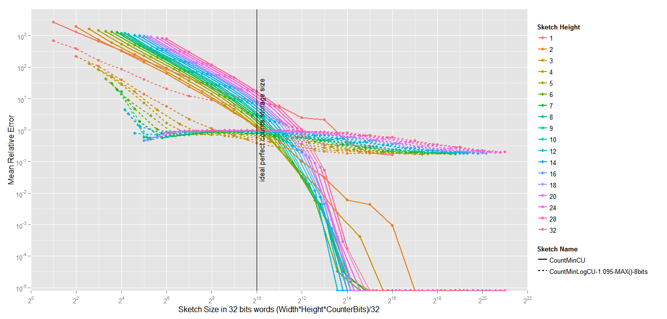
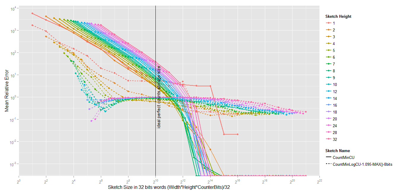
So I’ve introduced an interesting variation to the standard Count-Min Sketch, a variation which could, I think, be of high value for many uses, including mine. The idea is very simple, instead of using 32bits counters to count from 0 to 4294967295, we can use 8 bits counters to count from 0 to (approximately) 4294967295. This way, we can put 4 times more counters with the same number of bits, the risk of collisions is four times less, and thus, low frequency items are much less overestimated.
If you’re wondering how you can use a 8 bit counter to count from 0 to (approximately) 4294967295, just read this. It’s a log count using random sampling to increment the counter.
But it’s not all, first we can use the same very clever improvement to the standard Count-Min sketch which is called conservative update.
And additionaly, we can add a sample bias to the log-increment rule, which basically state that, if we’re at the bottom of the distribution, then probably we are going to be overestimated, then we should undersample.
Finally, we can have a progressive log base (for instance when the raw counter value is 1, the next value will be 1+1^1.1, but when the raw counter is 2, the next value will be 1+1^1.1+1^1.2). Zipfian distribution is not a power law, so why not go one step further..
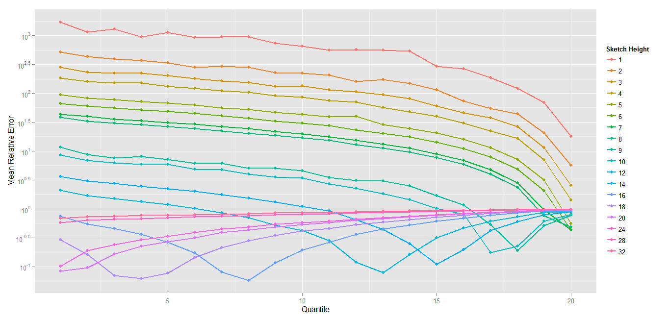
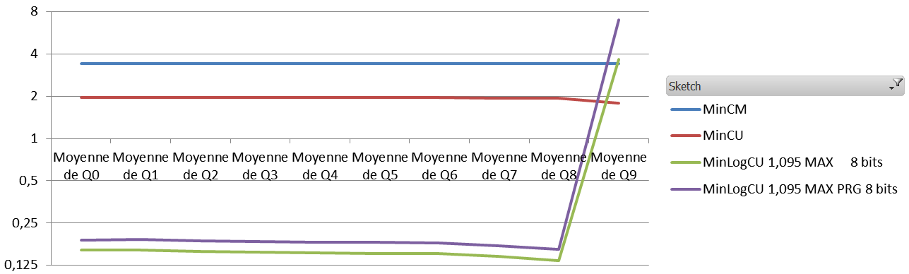
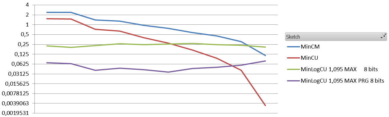
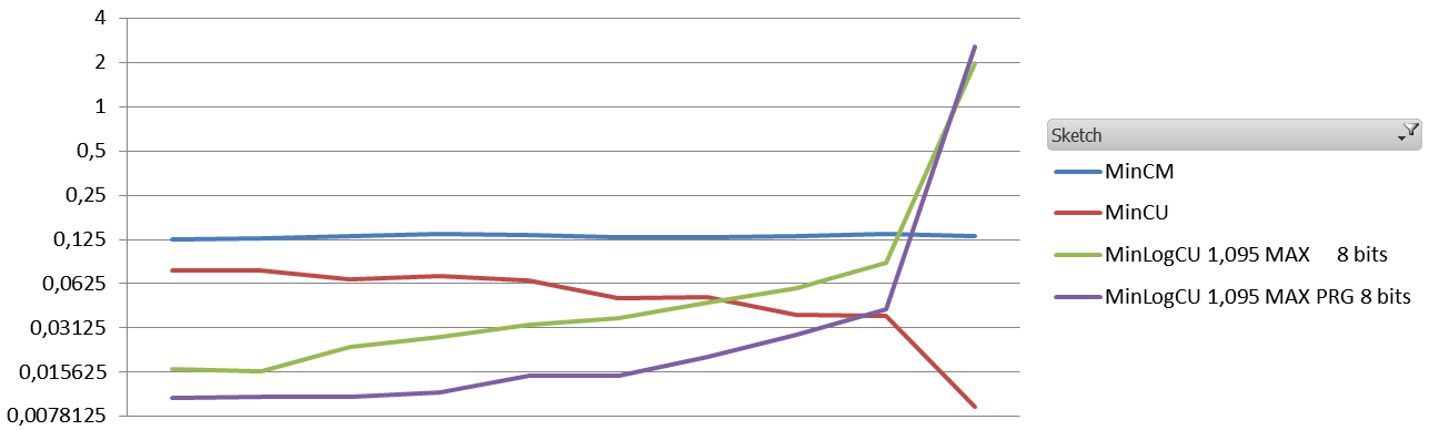
The results are quite interesting. Obviously the absolute error is way worst than the absolute error of a standard Count-Min. The Average Relative Error, however, is about 10 times less with different settings.
Here is the code :
1 2 3 4 5 6 7 8 9 10 11 12 13 14 15 16 17 18 19 20 21 22 23 24 25 26 27 28 29 30 31 32 33 34 35 36 37 38 39 40 41 42 43 44 45 46 47 48 49 50 51 52 53 54 55 56 57 58 59 60 61 62 63 64 65 66 67 68 69 70 71 72 73 74 75 76 77 |
import scala.util.Random import scala.util.hashing.MurmurHash3 /** * Created by guillaume on 10/29/14. */ class CountMinLogSketch(w:Int,k:Int,conservative:Boolean, exp:Double, maxsample:Boolean, progressive:Boolean, nBits:Int) { val store = Array.fill(k)(Array.fill(w)(0.toChar)) var totalCount = 0.0 val cMax = math.pow(2.0,nBits.toDouble) - 1.0 def value(c:Int, exp:Double):Double = { // For exp = 2, 0 -> 0, 1 -> 1, 2 -> 2, 3 -> 4, if (c == 0) 0.0 else math.pow(exp,c.toDouble-1.0) } def fullValue(c:Int, exp: Double):Double = { // For exp = 2, 0 -> 0, 1 -> 1, 2 -> 3, 3 -> 7 if (c <= 1) value(c, exp) else (1.0 - value(c+1, exp)) / (1.0 - exp) } def randomLog(c:Int, exp:Double) : Boolean = { // Return true with probability 1/(exp^(c+1)) // For exp = 2, 0 -> 1, 1 -> 1/2, 2 -> 1/4 val pIncrease = 1.0/(fullValue(c+1, getExp(c+1))-fullValue(c, getExp(c))) Random.nextDouble() < pIncrease } def getExp(c:Int) : Double = { if (progressive) 1.0 + ((exp - 1.0)*(c.toDouble - 1.0) / cMax) else exp } def getCount(s:String):Double = { val cl = (0 until k).map { i => store(i)(hash(s, i, w)) } val c = cl.min fullValue(c,getExp(c)) } def getProbability(s:String):Double = { val v = getCount(s) if (v > 0) getCount(s) / totalCount else 0 } def increaseCount(s:String):(Boolean,Double) = { totalCount += 1 val v = (0 until k).map { i => store(i)(hash(s, i, w)) } val vmin = v.min val c = if (maxsample) v.max else vmin assert(c <= cMax) val increase = randomLog(c, 0.0) if (increase) { (0 until k).map { i => val nc = v(i) if (!conservative || (vmin == nc)) { store(i)(hash(s, i, w)) = (nc + 1).toChar } } (increase, fullValue(vmin + 1, getExp(vmin + 1))) } else (false,fullValue(vmin, getExp(vmin))) } } |
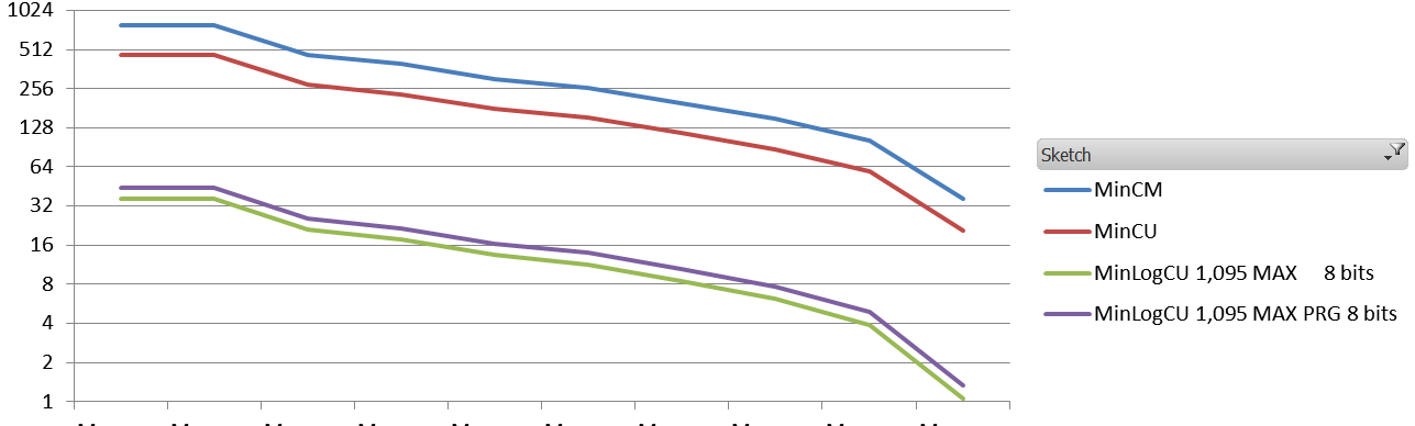
And the results (1.1 million events, 60K elements, zipfian 1.01, the sketches are 8 vectors of 5000*32 bits)
|
|---|
| Sketch |
Conservative |
Max Sample |
Progressive |
Base |
RMSE |
ARE |
| Count-Min |
NO |
- |
- |
- |
0.160 |
11.930 |
| Count-Min |
YES |
- |
- |
- |
0.072 |
6.351 |
| Count-MinLog |
YES |
YES |
NO |
1.045 (9 bits) |
0.252 |
0.463 |
| Count-MinLog |
YES |
YES |
YES |
1.045 (9 bits) |
0.437 |
0.429 |
| Count-MinLog |
YES |
YES |
NO |
1.095 (8 bits) |
0.449 |
0.524 |
| Count-MinLog |
YES |
YES |
YES |
1.095 (8 bits) |
0.245 |
0.372 |
| Count-MinLog |
YES |
YES |
NO |
1.19 (7 bits) |
0.582 |
0.616 |
| Count-MinLog |
YES |
YES |
YES |
1.19 (7 bits) |
0.677 |
0.405 |