eXenSa

I’ve been wondering for a while about the behaviour of SGNS vs SVD/PMI with regards to the difference of performance on analogy questions. (Have a look at Omer Levy’s TACL article  for a deep comparison of different methods).

One of my hypothesis is that, somehow, SGNS encodes the frequency of the words in its embedding. I think (haven’t tested it yet) that using frequency could help for many analogy questions, since one would expect, on average, that the frequency ratio between A and B is the same than between C and D.

One of the thing that made me think that SGNS could encode frequency is when I look at the neighbours of rare words :

With SVD (in parenthesis, the count from context with window size = 2):

1.0	iffy	(279)
0.809346555885	nitpicky	(125)
0.807352614797	miffed	(69)
0.804748781838	shaky	(934)
0.804201693021	sketchy	(527)
0.797617651846	clunky	(372)
0.794685053096	dodgy	(797)
0.792423714522	fishy	(494)
0.7876010544	listy	(211)
0.786528559774	picky	(397)
0.78497044497	underexposed	(73)
0.784392371301	unsharp	(130)
0.77507297907	choppy	(691)
0.770029271436	nit-picky	(90)
0.763106516724	fiddly	(43)
0.762200309444	muddled	(369)
0.761961572477	wonky	(196)
0.761783868043	disconcerting	(226)
0.760421351856	neater	(121)
0.759557240261	dissapointed	(32)

Variation : 0.1 – 3 x the query count

With SGNS :

1.0	iffy	(279)
0.970626	nitpicky	(125)
0.968823	bitey	(265)
0.968336	rediculous	(104)
0.967125	far-fetched	(262)
0.964707	counter-intuitive	(185)
0.964179	presumptuous	(126)
0.963679	disputable	(179)
0.963537	usefull	(183)
0.96175	clunky	(372)
0.96166	counterintuitive	(203)
0.961654	un-encyclopedic	(101)
0.961331	worrisome	(213)
0.960878	self-explanatory	(156)
0.960516	unecessary	(143)
0.960142	nit-picky	(80)
0.959044	wordy	(413)
0.958482	disconcerting	(226)
0.958218	disingenuous	(534)
0.958188	off-putting	(104)

Variation : 0.3 – 2 x the query count

That could actually be quite understandable. Since the update procedure of SGNS is online, the time of the update does have an importance (vectors at time t in the learning are not the same than at time t+s). So two rarely occuring words, if they occur roughly at the same time in the corpus, will tend to be updated by a few similar vectors (positively and negatively, by the way), and thus be highly influenced by the same direction of the data.

In other words, the rarer the word, the more its direction “lags behind” the rest of the embeddings, and in some way, the embedding slightly encodes the “age” of the words, and thus their frequency.

Here are its results on the same query with NCISC, with even more variation than SVD, with some apparently good high frequency candidates (debatable, unclear, unsatisfactory, questionable, and maybe wrong)  :

1.0	iffy	(279)
0.840267098681	debatable	(711)
0.835281154019	keepable	(67)
0.83013430458	disputable	(179)
0.821933628995	sketchy	(527)
0.813930181981	unsatisfactory	(1176)
0.812291787551	unclear	(4445)
0.804978094441	nitpicky	(125)
0.804038235737	us-centric	(170)
0.802013089227	dodgy	(797)
0.798211347285	salvagable	(118)
0.797837578971	shaky	(934)
0.797040400162	counter-intuitive	(185)
0.79600914212	ambigious	(41)
0.791063976199	offputting	(33)
0.789877149245	questionable	(6541)
0.789543971526	notible	(78)
0.786470266284	unconvincing	(567)
0.781320751203	wrong	(12041)
0.779762440213	clunky	(372)

Variation : 0.1 – 43 x query count

This excellent article  by Omer Levy, Yoav Goldberg and Ido Dagan give an amazingly detailed view on what is really behind Word2Vec method and GloVe success. I found it while reading comments on a Radim Rehurek’s post about Word2Vec.

Word2vec is one of the method which compete with our proprietary approach at eXenSa (the NCISC algorithm we use in eXenGine), even if it’s limited to words and documents. It produces very good embeddings.

What is truly impressive in the Levy et al. article is that they have dissected the algorithm to separate preprocessing choices (such as the word window or the count to weight transformation, which is basically Pointwise Mutual Information), algorithm parameters (for SVD, they show that removing the eigenvalues is always a good choice), and post-processing choices (for instance the distance computation for analogy tasks).

The only parameters they didn’t test is the number of target features. This is a bit odd, since that’s one of the selling point of NCISC, which performs very well even with 1/10 of the features required for Word2Vec, but can be easily explained since they already had to test something like 1000 different combinations.

As far as I can say, the most important piece of information from this article is that the choice of the method (raw PPMI, SVD, Word2Vec or Gradient Descent) does not play the biggest role in the final performance. It’s not really a surprise, since the main advantage of NN is in there non-linearity, and for text data, you basically already have too much dimensions to require dimensionality expansion.

 

 

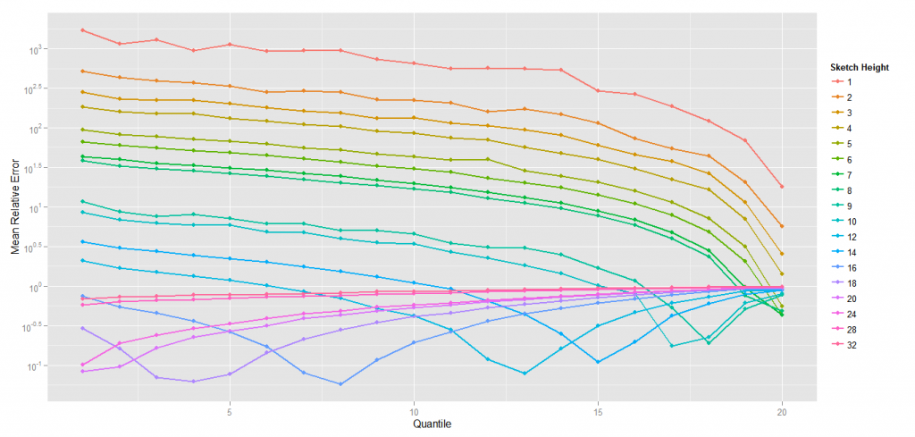
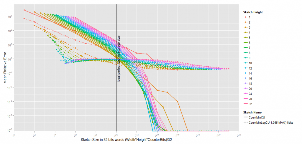
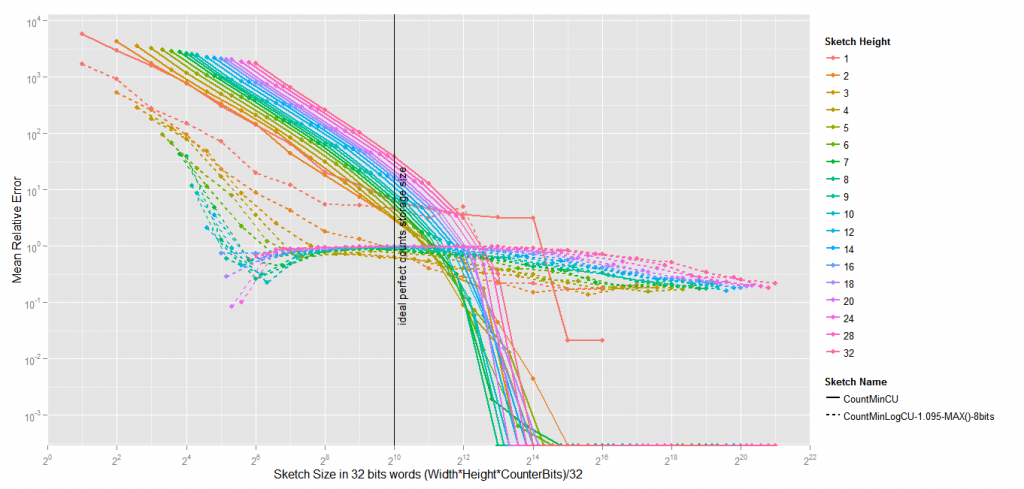
I’ve made a few experiments to have a look at the behaviour of the Count-Min-Log Sketch with Max sampling. Here are some interesting comparisons between classical Count-Min (the graphs show both the usual CM algorithm and the Conservative Update version), and Count-Min-Log.

For the sake of simplicity, I’ve chosen to limit to one setting in terms of memory use : in every sketch we use the same number of bits (here, 4 vectors of 4000*32 bits). I have also just shown the result of 8 bits Count-Min-Log (i.e. with base 1.095) with or without the progressive base (PRG).

Let’s start by the results under heavy pressure. Here we have 8 millions events in an initial vocabulary of 640,000 elements. The values are plotted for each decile of the vocabulary (i.e. on the left is the first 10th of the vocabulary with the lowest number of occurrences).

Now for the low pressure setting, still with 4 vectors of 4000*32bits for everyone, but this time the initial vocabulary is only 10000 and the number of events is about 100k.

 

Conclusion, for equal memory footprint, Count-Min-Log seems to clearly outperform classical Count-Min for high pressure settings, both for RMSE and ARE, with the exception of the RMSE for the top 10% highest frequency events. Under low pressure, it is clear that top 20-30% highest frequency items counts are significantly degraded.

I think that for any NLP-related task, Count-Min-Log is always a clear winner. For other applications, where the highest frequency are the most interesting, the gain may be negative, given the results on the high pressure setting. It will depend whether you care about ARE or RMSE.

Count-Min sketch is a great algorithm, but it has a tendency to overestimate low frequency items when dealing with highly skewed data, at least it’s the case on zipfian data. Amit Goyal had some nice ideas to work around this, but I’m not that fund of the whole scheme he sets up to reduce the frequency of the rarest cells.

I’m currently thinking about a whole new and radical way to deal with text mining, and I’ve been hitting repeatedly a wall while trying to figure out how I could be able to count the occurrences of a very very high number of different elements. The point is, what I’m interested in is abolutely not to count accurately the number of occurrences of high frequency items, but to get the order of magnitude.

I’ve come to realize that, using Count-Min (or, for that matter, Count-Min with conservative update), I obtain an almost exact count for high frequency items, but a completely off value when looking at low frequency (or zero-frequency) items.

To deal with that, I’ve realized that would should try to weight our available bits. In Count-Min, counting from 0 to 1 is valued as much as counting from 2147483647 to 2147483648, while, frankly, no one cares whether it’s 2147483647 or just 2000000000, right ?

So I’ve introduced an interesting variation to the standard Count-Min Sketch, a variation which could, I think, be of high value for many uses, including mine. The idea is very simple, instead of using 32bits counters to count from 0 to 4294967295, we can use 8 bits counters to count from 0 to (approximately) 4294967295. This way, we can put 4 times more counters with the same number of bits, the risk of collisions is four times less, and thus, low frequency items are much less overestimated.

If you’re wondering how you can use a 8 bit counter to count from 0 to (approximately) 4294967295, just read this. It’s a log count using random sampling to increment the counter.

But it’s not all, first we can use the same very clever improvement to the standard Count-Min sketch which is called conservative update.

And additionaly, we can add a sample bias to the log-increment rule, which basically state that, if we’re at the bottom of the distribution, then probably we are going to be overestimated, then we should undersample.

Finally, we can have a progressive log base (for instance when the raw counter value is 1, the next value will be 1+1^1.1, but when the raw counter is 2, the next value will be 1+1^1.1+1^1.2). Zipfian distribution is not a power law, so why not go one step further..

The results are quite interesting. Obviously the absolute error is way worst than the absolute error of a standard Count-Min. The Average Relative Error, however, is about 10 times less with different settings.

Here is the code :

And the results (1.1 million events, 60K elements, zipfian 1.01, the sketches are 8 vectors of 5000*32 bits)

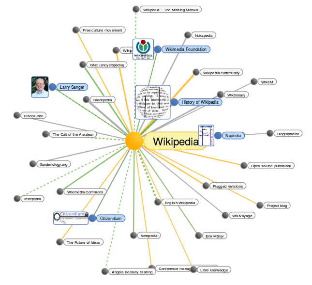
We’ve worked hard to make WikInsights more appealing and fun to use. Now it has a graphical interface with a graph view of the neighbours of Wikipedia.

Of course, the graph is dynamically generated and expose the most relevant neighbours along various dimensions, it’s not a view of the Wikipedia page graph.

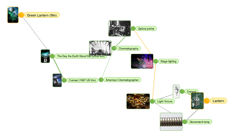
A very fun thing to do in wikinsights is to compute the similarity path between two pages. You can discover the path between the Green Lantern (movie) and a Lantern :

 

Have fun with it, and enjoy discovering new and relevant pages.

I gave a talk at the Paris Datageeks meetup a month ago. Here is the video of my presentation of Apache Spark.