Amazing results of NCISC on Netflix

Last week, I’ve played a little bit with the Netflix prize dataset and NC-ISC. The results are amazingly better than the current state of the art.

Short version

Netflix dataset contains ratings of movies by user. We try to predict unseen good ratings (a few ratings are kept aside in a separate dataset, and we try to see if we can predict that a given user would have rated those particular movies).

I’ve compared state-of-the-art results with my method, NC-ISC. With the best settings, I can predict 24% of the unseen ratings in the first 50 results, compared to 19% for the current best methods. Considering the fact that a non personalized prediction, based on popularity only, gives a 10% score, what we achieved is a 55% improvement over the current state of the art.

This is a huge gain.

And it could be applied to other recommendation problems : music, jobs, social network, products in e-commerce and social shopping, etc.

A bit of context

The Netflix Prize was an open competition held in 2009. The dataset consist of 100M ratings (1-5) given by 400K+ user on 17K+ movies. The original goal was to predict « unseen » ratings with the highest possible accuracy. The measure used was the RMSE (root mean square error) on the hidden ratings.

netflix-recommendations

The RMSE, however, is a very incomplete evaluation measure  (and also it cannot be estimated on the results of NC-ISC, which is one of the reason we haven’t spent much time to compare our results with the state of the art). Indeed, the common task for a recommender system is not to predict the rating you would give a given movie, but to provide you a list of K movies that you could potentially like.

As a result, more and more effort has been put on the so-called top-K recommender task, and as a side effect on learning to rank instead of learning to rate.

I’ve stumbled recently on an interesting paper : Alternating Least Squares for Personalized Ranking by Gabor Takacs and Domonkos Tikk, from RecSys 2012 (which has been covered here), and found myself happy to find a paper with results I could compare to (often, either the metric, or the dataset is at odds with what I can produce/access).

The experiment

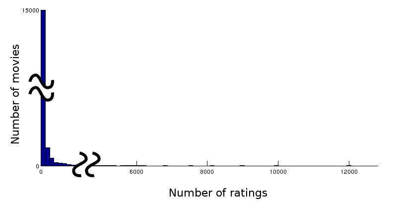
So I ran NC-ISC on the same dataset they used in the paper (just keep the top ratings), which reduce the train dataset to 22M ratings and the probe to 400K ratings. At first the results were very disappointing. The main reason for this is that NC-ISC inherently discards any bias on popularity. And the fact is, ranking Movies is a very popularity-biased problem (below we can see that 15000 movies have very few ratings in the test set, while a few movies have 12000 ratings) :

Distribution Ratings Netflix

However, while NC-ISC cannot perform rating prediction natively, and discards popularity in both its learning and its ranking, it’s quite easy to put popularity back into the learning, and back into the ranking. Putting it back in the ranking simply means to multiply the score produced by NC-ISC by each movie popularity. Putting popularity back into the learning means decreasing the unbiasing factor in NC-ISC.

The results

And here we come (I’ve added my results as an overlay to the original paper figure). Just a disclaimer : while I’ve reproduced results from the popularity baseline, I didn’t have the time to check the implicit ALS results (I’ve got an implementation here in Octave that take hours to run), so I’m not 100% confident I haven’t missed something in the reproduction of the experiment.

NetFlix-Recall@50

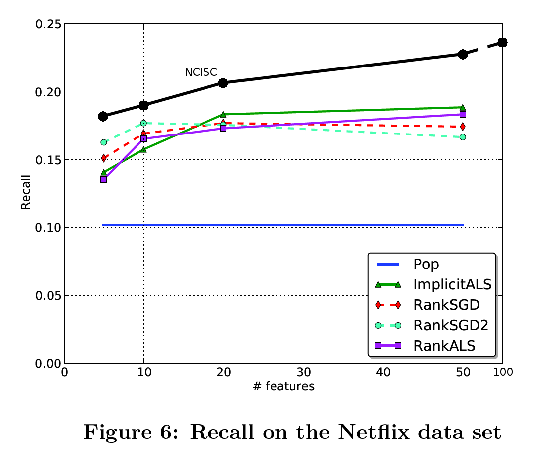
I’ve added a mark for 100 features, which wasn’t in the original paper, probably since there results tended to stop improving.

Performance

A short note about NCISC performance versus ImplicitALS, RankALS and RankSGD. First, while SGD takes on average 30 iterations to converge, ALS and NCISC takes between 5 and 10 iterations.

Regarding iteration time, while Takacs and Tikk give their timings for Y!Music data, I could only work top Netflix ratings dataset. However, the two datasets have approximately the same number of ratings (22M) and approximately the same total number of elements (17700 + 480189 = 497889 for Netflix, 249012+296111= 545123 for Y!Music).

Finally, I’ve run my unoptimized algorithm using 1 core of a Core i7 980 (cpumark score 8823 for 6 cores), while they have used 1 core of a Xeon E5405  (2894 for 4 cores) to run their unoptimized RankALS and ImplicitALS and optimized RankSGD algorithms. The rescaling factor to account for the processor difference is thus exactly 2 (!)

Here are my rescaled timings and the original timings of the other methods (remember it’s not an optimized version, though):

method #5 #10 #20 #50 #100
NC-ISC 1 2 4 10 25
ImplicitALS 82 102 152 428 1404
RankALS 167 190 243 482 1181
RankSGD 21 25 30 42 65
RankSGD2 26 32 40 61 102

 Time (seconds) per iteration for various # of features.

Speedup range from x3 to x167 per iteration (for SGD you should account for the increased number of iterations required). I’ve generally observed that my optimized implementations of NC-ISC run 10 to 20 times faster than my Matlab implementation.

More features, more results on wikipedia

While we are working to make eXenGine more efficient, more expressive and, more specifically more sellable, I keep playing with the results of NCISC on Wikipedia. Here is an example of the neighbours of GenSim (a well known python toolkit for text mining/natural language processing by Radim Řehůřek), this time on the document/word model with 90 features :

  • OpenNLP : 0.9343325
  • Semantically-Interlinked Online Communities : 0.92996
  • GML Application Schemas : 0.9280249
  • XML Metadata Interchange : 0.926392
  • Languageware : 0.924556
  • Visual modeling : 0.92413026
  • GeoSPARQL : 0.9231725
  • Clairlib : 0.92301136
  • Heurist : 0.92240715
  • VisTrails : 0.9223076
  • Embedded RDF : 0.92183596
  • NetworkX : 0.9217739
  • UIMA : 0.9217461
  • Software Ideas Modeler : 0.92173994
  • List of Unified Modeling Language tools : 0.9215104
  • UModel : 0.92115307
  • SmartQVT : 0.9210423
  • Linked data : 0.9207388
  • Natural Language Toolkit : 0.92064124

It’s far from perfect, one major cause being that we still don’t use bigrams or skip-grams in the input transformation (i.e. we use plain old style bag of words), but it clearly shows the power of NCISC.

You can compare with the results provided by LSA using GenSim itself, in this post, a comment gives the top 10 results on a 500 features model trained on wikipedia:

  • Snippet (programming)
  • Prettyprint
  • Smalltalk
  • Plagiarism detection
  • D (programming language)
  • Falcon (programming language)
  • Intelligent code completion
  • OCaml
  • Explicit semantic analysis

When using the document/document interlink model (90 features), we obtain different, very good results:

  • Jubatus : 0.98519164
  • Scikit-learn : 0.98126435
  • Feature Selection Toolbox : 0.97841007
  • Structure mining : 0.97700834
  • ADaMSoft : 0.9755426
  • Mallet (software project) : 0.97395116
  • Shogun (toolbox) : 0.9718502
  • CRM114 (program) : 0.96751755
  • Weka (machine learning) : 0.96635485
  • Clairlib : 0.9659551
  • Document retrieval : 0.96506816
  • Oracle Data Mining : 0.96350515
  • Approximate string matching : 0.96212476
  • Bayesian spam filtering : 0.96208096
  • Dlib : 0.9620419
  • GSP Algorithm : 0.96116054
  • Discounted cumulative gain : 0.9606682
  • ELKI : 0.9604578
  • NeuroSolutions : 0.96015286
  • Waffles (machine learning) : 0.9597046
  • Information extraction : 0.9588822
  • Latent semantic mapping : 0.95838064
  • ScaLAPACK : 0.9563968
  • Learning Based Java : 0.95608145
  • Relevance feedback : 0.9559279
  • Web search query : 0.9558407
  • Grapheur : 0.9556832
  • LIBSVM : 0.95526296
  • Entity linking : 0.95325243

Much better than the 40 features version displayed on our demo site,

  • Java GUI for R : 0.995283
  • Decision table : 0.99500793
  • Programming domain : 0.9946934
  • Scikit-learn : 0.994619
  • Feature model : 0.9941954
  • Dlib : 0.9938446
  • Pattern directed invocation programming language : 0.9937961
  • Compiler correctness : 0.9937197
  • On the Cruelty of Really Teaching Computer Science : 0.99280906
  • Structure mining : 0.99274904
  • Hidden algebra : 0.99265593
  • OMDoc : 0.9925574
  • Institute for System Programming : 0.99253553
  • Radial tree : 0.9924036
  • Partial evaluation : 0.9922968
  • Jubatus : 0.99167436
  • Query optimization : 0.9916388
  • Effect system : 0.99141824


Spark + MLLib

Spark with a star
Apache Spark Logo

I’m still digging into Spark and MLLib, but for now, I can clearly say that this combination has some serious points.

  • It can easily replace PIG with the added benefit that you don’t have to mix several technologies for you UDFs
  • It’s really efficient
  • It’s made for iterative methods (which is the case for NC-ISC) and definitely more suited for ML than pure Hadoop/MRv1 (I don’t know if Yarn performs better, but I don’t really think so)
  • Scala is a great language
  • Spark is at least as scalable as Hadoop, and can use several cluster management systems : Hadoop Yarn, EC2, Mesos and Spark

My opinion is that Spark is the near-perfect framework to efficiently write efficient mapreduce jobs (see the double efficiency here ?)

Also, it’s funny to see that Twitter’s Scalding has partially the same goal as Spark (i.e. help writing concise MapReduce jobs) except that Spark adds a much more powerful execution engine that allows intermediate computations to be kept in memory when possible. Probably not something that really big datasets can afford, but at least it’s a good thing to have it as an option.


Reuters 21578 dataset : inconsistent results

I have recently decided to take a quick look back to a problem I haven’t spent much time to solve, namely my results on the Reuters dataset. One of my problems was due to inconsistent results between my experiments and the published results by Ranzato and Szummer.

I have already talked about their paper in previous posts, and NC-ISC outperforms their method on the 20 newsgroups dataset (they haven’t published any precision/recall curve on Ohsumed). On the small Reuters dataset, though, they have very good results, and they also publish some material that I have a hard time reproducing. The figure 4 of their paper « Semi-supervised learning of compact document representations with deep networks », especially, compares results from LSI and from their method. The problem is that my own experiments show much better results for LSI.

Their results :

Screenshot-Semi-supervised_Learning_of_Compact_Document_Representations_with_Deep_Networks


And my results (just LSI) :

reuters-LSI

To sum up : my results for LSI-2 starts with a precision of 0.35 while theirs starts with a precision of 0.06, LSI-10 respectively starts at 0.57 versus 0.35, and LSI-40 at 0.68 versus 0.56.

What is really surprising (even though, technically, not completely impossible) is that their results for LSI-2 and LSI-3 are below the baseline one could obtain by randomly choosing documents. My TF-IDF curve is relatively close to theirs (even though not exactly the same).

Since they have taken the data from the same source I have, I really don’t understand how we can have such different results.

Another puzzling fact is that, on the Reuters dataset, TF-IDF actually performs worse than cosine distance on the raw counts (at least for a recall below 1%). This is, I think, the only dataset with such a behaviour.


Recent NC-ISC method improvement

Despite the already good results of our method, we have further improved it. The most notable improvement is due to a better handling of the numeric compatibility between the two final embeddings (for instance words and documents embedding).

Here are the results on 20newsgroups-bydate (60% training, 40% testing, test data correspond to the latest documents in time).

This was also the occasion for us to show how simply injecting  »a priori » knowledge about word semantics can significantly improve the results (this  »a priori » knowledge is computed using NC-ISC on a cooccurrence matrix, using a 20 words window on a mix of 20newsgroups and reuters RCV1 corpus).

The curves are classical precision/recall results. For comparison, I have included what I think are the best results in the state of the art (I have missed more recent results, please tell me) from Ranzatto & Szummer (ICML 2008) from their figure showing their best results of the shallow method (I have no clue as to whether their deep method can do any better, but I doubt it since they mainly argue that deep methods can perform as well as shallow method but with less features).

NC-ISC-small-old

One interesting thing is that Ranzatto and Szummer use a preprocessed 20 newsgroups corpus that reduce their vocabulary to 10000 (using Rainbow), while we use pure raw words (including uppercase and lowercase variants). It would be interesting to see wether their method could perform better if they were to use the whole unprocessed vocabulary. Also, our first experiments using frequent pairs and triplets of words as new vocabulary items has shown an unexpected global performance decrease (this concern raw TF-IDF as well as all NC-ISC variants). Comments on this are warmly welcome.